Google Meridian Adstock and Hill Saturation: How It Differs From the Standard Formula
Almost every MMM tutorial teaches adstock as a recursive carryover formula. Google Meridian does not implement that formula. The difference changes what your decay rate means, how half-life should be computed, and whether your Hill saturation parameters are interpretable at all.
 Mohit Luthra
16 min
Mohit Luthra
16 min
If you have read three blog posts about marketing mix modelling, you have seen the same adstock formula three times: this week's advertising pressure equals this week's spend plus a fraction of last week's pressure. It is recursive, it is elegant, and it is what most open-source MMM code actually runs.
Google's Meridian does not use it. Meridian computes a bounded, normalised weighted average over a fixed lag window. Mathematically these are cousins, not twins, and the differences are not academic. They change what α means, what your half-life calculation is telling you, and whether the saturation parameter sitting next to it is interpretable at all.
This post walks the whole path: what adstock is and why MMM needs it, the traditional recursion and its half-life arithmetic, what Meridian actually implements, how the Hill function handles saturation, and what you gain and lose by switching.
What adstock is, and why a regression needs it
Advertising does not stop working when it stops running. A television flight that ends on Sunday is still producing sales on Wednesday. People saw the ad, did not act immediately, and acted later.
This breaks a naive regression in a specific and predictable way. Suppose you run a four-week burst and then go dark:
| Week | TV spend | Sales |
|---|---|---|
| 1-4 | ₹10L/week | elevated |
| 5-8 | ₹0 | still elevated, drifting down |
| 9+ | ₹0 | back to baseline |
Regress weekly sales on weekly TV spend and the model sees spend in weeks 1-4 and zero in weeks 5-8. It also sees elevated sales in weeks 5-8 that it cannot attribute to TV, because TV spend is zero there. So it does one of two things: shrinks the TV coefficient toward zero, or hands the credit to whatever variable happened to be non-zero in those weeks.
That second failure mode is the reason branded search posts absurd ROI in badly specified models. Search spend is always on. When brand media creates demand that shows up as a search query two weeks later, an un-adstocked model has no mechanism to trace it back, so search collects the credit. The coefficient is not wrong arithmetically. The specification is wrong.
Adstock fixes this by replacing spend with a stock: a constructed variable representing how much advertising pressure is still in the market this week, combining current spend with a decayed remainder of previous weeks.
The traditional recursion
The workhorse specification, the one in most tutorials and most open-source libraries:
One parameter. λ is the decay rate. At \lambda = 0 the stock collapses to raw spend. At \lambda = 0.9, nine-tenths of the pressure survives each week and a single burst echoes for months.
Because the recursion is geometric, it has a closed form as an infinite weighted sum of lagged spend:
Two quantities fall out of λ directly, and both are worth reporting to stakeholders who will never look at a coefficient table.
At \lambda = 0.76: half-life of 2.5 weeks, and one rupee of spend generates 4.2 rupees of cumulative adstock. That second number is the one that causes trouble.
The recursion inflates the regressor by 1/(1-\lambda), and by a different factor for every channel. TV at 0.76 gets multiplied by 4.2×; search at 0.37 gets 1.6×. If you fit coefficients on un-normalised adstock, those coefficients are not comparable across channels, and your contribution decomposition inherits the distortion. Most implementations handle this by dividing through by 1/(1-\lambda). Many do not, and it is worth checking the one you use.
Below is the transform applied to a single four-week burst. Drag decay to see carryover stretch, and switch presets to compare channels.
The Search preset is the instructive one. At \lambda = 0.37 the stock is nearly indistinguishable from the spend line, which is exactly right. Someone searching for a product has intent now; there is very little pressure left in the market two weeks later. Television is the opposite, and the gap between those curves is the whole argument for why you cannot evaluate both channels on a same-week attribution window.
What Meridian actually computes
Here is where the tutorials and the library diverge. Meridian's adstock is a normalised weighted average over a finite lag window, not an unbounded recursion:
Three structural differences from the recursion.
It is bounded. L (max_lag in the API) caps how far back the window reaches. The recursion technically looks back forever; Meridian looks back exactly L periods and stops. You choose L, the model does not learn it.
Set the recursion to Raw and the scale gap is immediate: at α = 0.76 and L = 8, the recursion peaks near 278 while Meridian peaks around 73, because Meridian is averaging where the recursion is summing. Meridian's peak sits below the 100-unit spend line, which surprises people the first time. It is correct: a four-week burst inside an eight-week window means half the window is zeros, and they pull the average down. Switch to Normalised and the peaks align, but the shapes still differ, and shrinking max_lag pulls Meridian's tail in while the recursion keeps trailing regardless. That last behaviour is the one worth sitting with: max_lag is a real modelling lever in Meridian, and has no counterpart in the recursion at all.
It is normalised by construction. Dividing by \sum w(s;\alpha) means the output is a weighted average of recent spend, not a weighted sum. Adstocked TV and adstocked search come out on the same scale as their raw inputs, and as each other. The scale problem from the previous section does not exist here; it is designed out.
The weight function is pluggable. Meridian ships two. Geometric is the familiar one:
Binomial is the one people miss:
The practical difference: geometric weights approach zero but never reach it, so the choice of L is a truncation of something still positive. Binomial weights go to zero at s = L, making the window boundary a real feature of the curve rather than an arbitrary cut. For channels with a genuine finite memory, binomial is the more honest shape.
The two curves separate most at the far end of the window. Geometric still assigns real weight to lag L, so truncating there throws away pressure the model believes exists. Binomial has already gone to zero, which means L is describing the channel rather than cutting it off.
Meridian learns α, ec, and slope from the data, with priors. You set max_lag and the decay function type. This split matters when someone asks why the model "chose" an 8-week window. It did not. You did.
Why normalisation is not a detail
This is the point I would most want a reader to leave with, because it connects adstock to the saturation stage sitting immediately after it.
Meridian's saturation is a two-parameter Hill function:
ec is defined as the input level at which response reaches half its ceiling. That definition is only useful if you know what scale the input is on. Feed Hill an un-normalised adstock and ec is expressed in units of "spend times an arbitrary channel-specific multiplier", which is not a quantity anyone can reason about or set a prior over.
Because Meridian normalises, the adstock handed to Hill is on the scale of media units per capita. So ec is too. It becomes a number a media planner can actually interpret: the exposure level at which this channel is half-saturated.
The concave preset is what Meridian's default prior expects. Switch to S-shaped and look at the region below ec: the curve is convex there, meaning the second rupee returns more than the first. That is a real phenomenon in some categories, and it is also what makes budget optimisation misbehave, because a convex region gives the optimiser an incentive to pile spend into a channel until it crosses the inflection.
spend → adstock (bounded, normalised) → Hill saturation → coefficient. Each arrow is a modelling choice you should be able to defend. Meridian's default applies Hill after adstock — controlled by hill_before_adstock=False — which means saturation acts on accumulated pressure rather than on each week's spend in isolation. That ordering is the defensible one: diminishing returns should respond to how much pressure is in the market, not to how much you happened to spend last Tuesday.
On the slope parameter, one practical warning. Values at or below 1 give a concave curve. Above 1 you get an S-shape, convex below ec and concave above it. Meridian's default prior assumes concave, and for good reason: convex regions break the assumptions most budget optimisers rely on, and can cause convergence problems during sampling. If you find yourself reaching for an S-curve, be sure you have the data to identify it.
The code
Meridian's transforms are exposed directly, so you can apply them outside a full model fit. Useful for building intuition or for sanity-checking a fitted parameter against what you expected.
import numpy as np
from meridian.model.adstock_hill import AdstockTransformer, HillTransformer

# media shape: [n_geos, n_media_times, n_channels]
media = np.random.gamma(2.0, 1.5, size=(1, 104, 4)).astype("float32")

# alpha shape: [n_channels] -- one decay rate per channel
alpha = np.array([0.76, 0.69, 0.63, 0.37], dtype="float32")

adstock = AdstockTransformer(
    alpha=alpha,
    max_lag=8,                    # L: you set this, the model does not learn it
    n_times_output=104,
    decay_functions="geometric",  # or "binomial", or a per-channel list
)
stock = adstock.forward(media)

# ec and slope shape: [n_channels]
hill = HillTransformer(
    ec=np.array([2.1, 1.8, 1.4, 0.9], dtype="float32"),
    slope=np.array([0.9, 1.0, 0.8, 1.1], dtype="float32"),
)
response = hill.forward(stock)

print(media.mean(), stock.mean(), response.mean())
# stock.mean() sits close to media.mean() -- that is normalisation working
Mixing decay functions per channel is a one-line change, and worth doing when channel memory genuinely differs in shape:
from meridian.model.adstock_hill import AdstockDecaySpec

# TV and print have a real finite memory; digital trails off asymptotically
spec = AdstockDecaySpec(
    media=["binomial", "binomial", "geometric", "geometric"],
)

# or, the simple case
spec = AdstockDecaySpec.from_consistent_type("geometric")
To reproduce the half-life intuition under Meridian's normalised weights, compute it from the weights themselves rather than from the closed form. The closed-form \ln 0.5 / \ln \lambda assumes the unbounded recursion, and will be wrong by a small but real amount once the window is truncated:
def weighted_half_life(alpha: float, max_lag: int = 8) -> float:
    """Half-life implied by Meridian's normalised geometric weights."""
    lags = np.arange(max_lag + 1)
    w = alpha ** lags
    w = w / w.sum()
    cumulative = np.cumsum(w)
    return float(np.searchsorted(cumulative, 0.5))
Diagnostics that are worth reading
Two plots do most of the work when you are checking whether the transforms behaved.
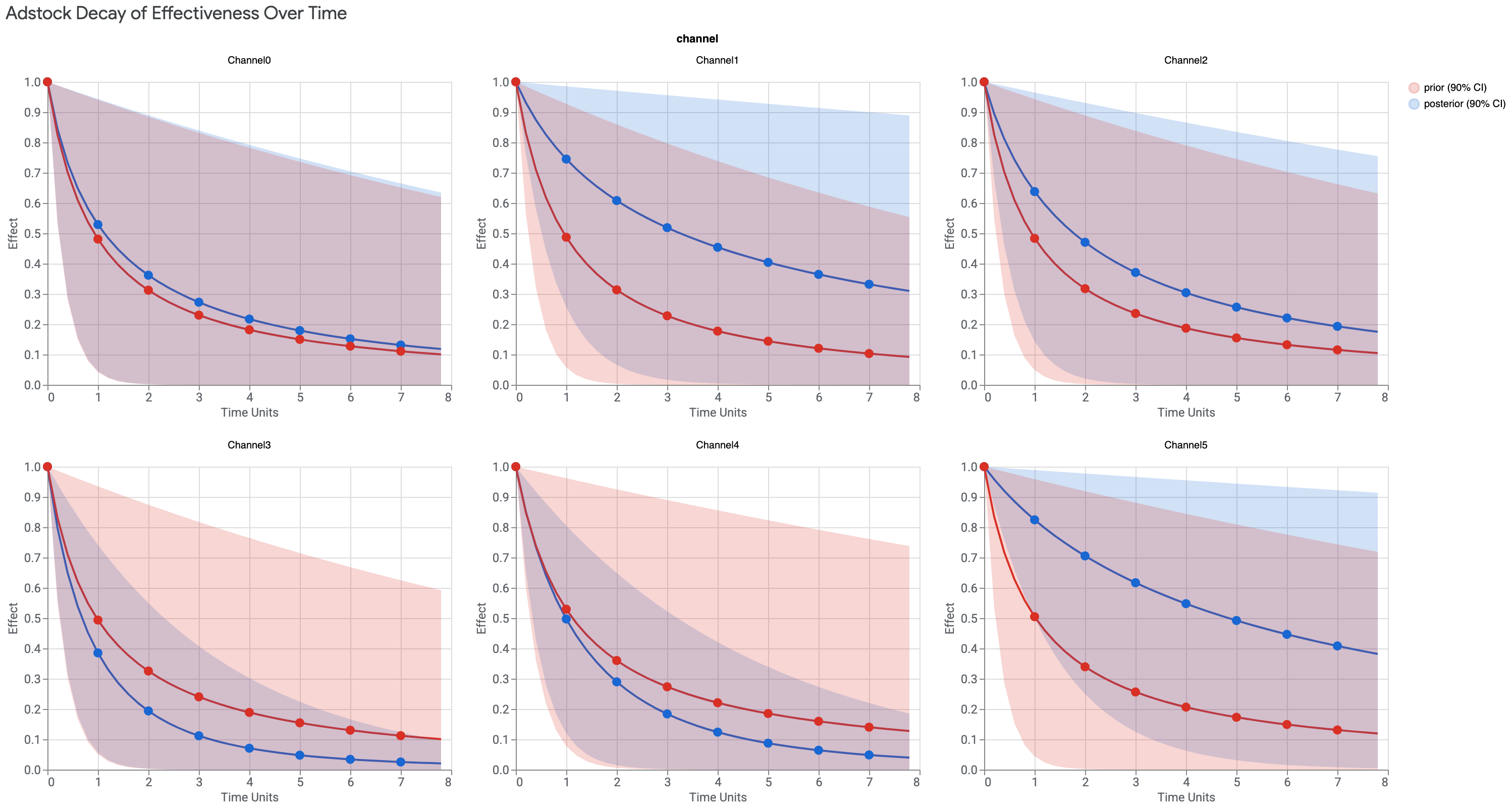
α for that channel, and you should not build a reallocation argument on it.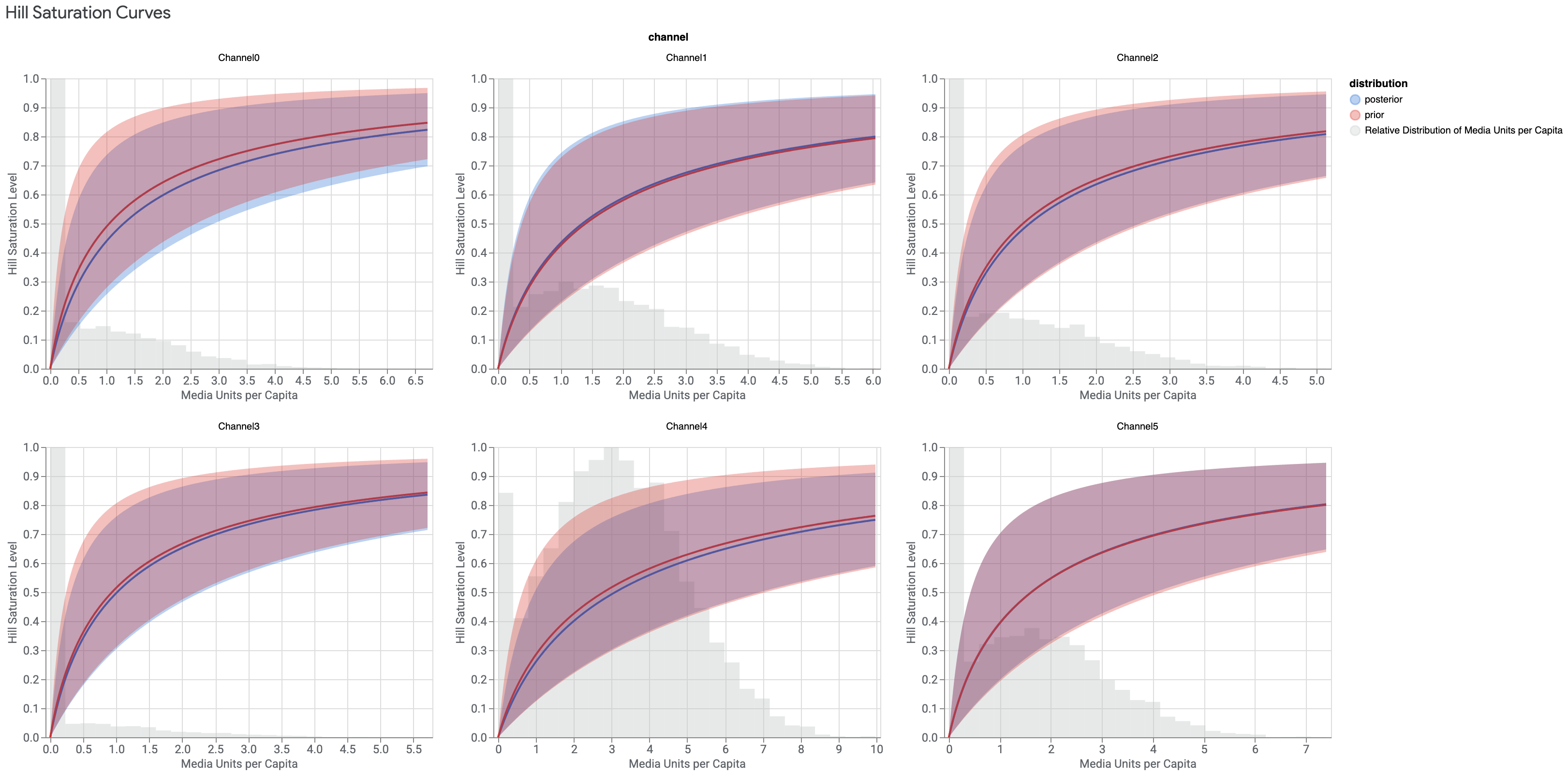
That second point generalises. Meridian fits Hill parameters from the observed range of media data. The curve extends past that range because it is a continuous function, not because the model knows anything about what happens there.
Trade-offs, honestly
What the bounded weighted average gives you. Channels are comparable without a manual normalisation step. ec means something. The lag window is an explicit, documented assumption rather than an implicit consequence of the functional form. Two decay shapes instead of one. All of this is engineered to hold together as a system.
What it costs you. Your α is not directly comparable to a λ from a recursive implementation, and the standard half-life formula does not transfer cleanly. max_lag becomes a decision you own, and a wrong one truncates real carryover with no warning in the output. The Bayesian fit is slower than a grid search by a wide margin. And the normalised form makes "total multiplier applied to a rupee of spend" a less natural quantity to extract, which is a genuine loss when you are presenting to a finance team who liked that number.
When the recursion is still the right call. Fast iteration, small datasets, or a stakeholder group that already thinks in half-lives. Just be explicit about which one you ran, and normalise before you compare channels.
The two formulas are not competitors, they solve the carryover problem in different ways, and both are mathematically sound. What matters is knowing which one is actually running under the hood, because the reporting language changes with it: a half-life quoted from Meridian output should be computed from Meridian's normalised weights, not pulled from the textbook closed form. Once that link between the formula and the language describing it is solid, the rest of the model becomes much easier to explain to a stakeholder who has never seen either equation and never needs to.